R: 使用公共数据库构建癌症预后模型

## If you need to download other cancers, simply replace TCGA-LIHC with the corresponding cancer abbreviation in the first line.

proj <- “TCGA-LIHC”

download.file(url = paste0(“https://gdc.xenahubs.net/download/”,proj, “.htseq_counts.tsv.gz”),destfile = paste0(proj,”.htseq_counts.tsv.gz”))
download.file(url = paste0(“https://gdc.xenahubs.net/download/”,proj, “.GDC_phenotype.tsv.gz”),destfile = paste0(proj,”.GDC_phenotype.tsv.gz”))
download.file(url = paste0(“https://gdc.xenahubs.net/download/”,proj, “.survival.tsv”),destfile = paste0(proj,”.survival.tsv”))

## Import expression matrix and clinical data

clinical = read.delim(paste0(proj,”.GDC_phenotype.tsv.gz”),fill = T,header = T,sep = “\t”)
surv = read.delim(paste0(proj,”.survival.tsv”),header = T)
dat = read.table(paste0(proj,”.htseq_counts.tsv.gz”),check.names = F,row.names = 1,header = T)

## Organize the expression matrix and take the logarithm of counts.

dat <- as.matrix(2^dat – 1)
exp <- apply(dat, 2, as.integer)
rownames(exp) <- rownames(dat)
library(AnnoProbe)
library(stringr)
rownames(exp) = str_split(rownames(exp),”\\.”,simplify = T)[,1];head(rownames(exp))
re = annoGene(rownames(exp),ID_type = “ENSEMBL”);head(re)
library(tinyarray)
exp = trans_array(exp,ids = re,from = “ENSEMBL”,to = “SYMBOL”)

##Data filtering was performed to retain only the genes expressed in at least half of the samples.

exp = exp[apply(exp, 1, function(x) sum(x > 0) > 0.5*ncol(exp)), ]

###Differentiation and grouping of cancer and adjacent non-cancer samples were performed based on barcodes.

Group = ifelse(as.numeric(str_sub(colnames(exp),14,15)) < 10,’tumor’,’normal’)
Group = factor(Group,levels = c(“normal”,”tumor”))
table(Group)# View the number of each group

### Filter out normal samples, leave only cancer samples, and convert them to logCPM format

exprSet=log2(edgeR::cpm(exp[,Group==’tumor’])+1)

###Integration of clinical data.

library(dplyr)
meta <- left_join(surv,clinical,by = c(“sample”= “submitter_id.samples”))
k = meta$sample %in% colnames(exprSet);table(k)
meta = meta[k,]
k1 = meta$OS.time >= 30;table(k1)
k2 = !(is.na(meta$OS.time)|is.na(meta$OS));table(k2)
meta = meta[k1&k2,]

tmp = data.frame(colnames(meta))

meta = meta[,c(
‘sample’,
‘OS’,
‘OS.time’,
‘race.demographic’,
‘age_at_initial_pathologic_diagnosis’,
‘gender.demographic’ ,
‘tumor_stage.diagnoses’,
‘pathologic_T’,
‘pathologic_N’,
‘pathologic_M’
)]

dim(meta)# View dimension information of the matrix

rownames(meta) <- meta$sample

meta[1:4,1:4]# View the column names of the matrix

colnames(meta)=c(‘ID’,’event’,’time’,’race’,’age’,’gender’,’stage’,’T’,’N’,’M’)# Simplify column names for meta.

meta[meta==””|meta==”not reported”]=NA
s = intersect(rownames(meta),colnames(exprSet))
exprSet = exprSet[,s]
meta = meta[s,]

identical(rownames(meta),colnames(exprSet))

#Multivariate Cox regression analysis

library(survival)
coxfile = paste0(proj,”_cox.Rdata”)
if(!file.exists(coxfile)){
cox_results <-apply(exprSet , 1 , function(gene){
meta$gene = gene
meta$group=ifelse(gene>median(gene),’high’,’low’)
meta$group = factor(meta$group,levels = c(“low”,”high”))
m=coxph(Surv(time, event) ~ group, data = meta)
beta <- coef(m)
se <- sqrt(diag(vcov(m)))
HR <- exp(beta)
HRse <- HR * se
#summary(m)
tmp <- round(cbind(coef = beta,
se = se, z = beta/se,
p = 1 – pchisq((beta/se)^2, 1),
HR = HR, HRse = HRse,
HRz = (HR – 1) / HRse,
HRp = 1 – pchisq(((HR – 1)/HRse)^2, 1),
HRCILL= exp(beta – qnorm(.975, 0, 1) * se),
HRCIUL = exp(beta + qnorm(.975, 0, 1) * se)), 3)
#return(tmp[‘gene’,])
return(tmp[‘grouphigh’,])
})
cox_results=as.data.frame(t(cox_results))
save(cox_results,file = coxfile)
}
load(coxfile)# Load calculation results

# Count the number of genes with p-values less than 0.01
table(cox_results$p<0.01)
# Count the number of genes with p-values less than 0.05
table(cox_results$p<0.05)

#Logrank test analysis

logrankfile = paste0(proj,”_log_rank_p.Rdata”)
if(!file.exists(logrankfile)){
log_rank_p <- apply(exprSet , 1 , function(gene){
meta$group=ifelse(gene>median(gene),’high’,’low’)
data.survdiff=survdiff(Surv(time, event)~group,data=meta)
p.val = 1 – pchisq(data.survdiff$chisq, length(data.survdiff$n) – 1)
return(p.val)
})
log_rank_p=sort(log_rank_p)
save(log_rank_p,file = logrankfile)
}
# Load calculation results
load(logrankfile)
# Count the number of genes with p-values less than 0.01
table(log_rank_p<0.01)
# Count the number of genes with p-values less than 0.05
table(log_rank_p<0.05)

#Import the gene set of interest, only the gene symbols are needed

Sc_TIME_Diff<- read.table(“./data/diff1.csv”, sep = “,”,header = T, row.names = 1)
Sc_TIME_Diff <- rownames(Sc_TIME_Diff)
hsa04979_diff<- read.table(“./data/diff2.csv”,sep = “,”,header = T,row.names = 1)
hsa04979_diff <- rownames(hsa04979_diff)
all <- c(Sc_TIME_Diff, hsa04979_diff)
cox005 = rownames(cox_results)[cox_results$p<0.05];length(cox005)
model_list <- intersect(all,cox005)

#Construct a prognostic model.

exprS = exprSet[model_list,]
x=t(exprS)# Row name is sample, column name is gene
y=meta$event
library(glmnet)
set.seed(123456) # Set random seeds
# Does k-fold cross-validation for glmnet, produces a plot, and returns a value for lambda
cv_fit <- cv.glmnet(x=x, y=y)
plot(cv_fit)
fit <- glmnet(x=x, y=y)
plot(fit,xvar = “lambda”)
model_lasso_min <- glmnet(x=x, y=y,lambda=cv_fit$lambda.min)
model_lasso_1se <- glmnet(x=x, y=y,lambda=cv_fit$lambda.1se)
choose_gene_min=rownames(model_lasso_min$beta)[as.numeric(model_lasso_min$beta)!=0]
choose_gene_1se=rownames(model_lasso_1se$beta)[as.numeric(model_lasso_1se$beta)!=0]
length(choose_gene_min)
length(choose_gene_1se)
lasso.prob <- predict(cv_fit, newx=x , s=c(cv_fit$lambda.min,cv_fit$lambda.1se) )
lasso_riskscore <- predict(cv_fit, newx=x , s=cv_fit$lambda.min,type=”link”)
re=cbind(y ,lasso.prob)
head(re)
re=as.data.frame(re)
colnames(re)=c(‘event’,’prob_min’,’prob_1se’)
re$event=as.factor(re$event)
g = choose_gene_min
e=t(exprS[g,])
library(stringr)
colnames(e)= str_replace_all(colnames(e),”-“,”_”)
dat1=cbind(meta,e)
colnames(dat1)
library(survival)
library(survminer)
dat2 = na.omit(dat1)
dat2 <- dat1[,-1]
dat2 <- dat2[,-(3:9)]
#vl <- colnames(dat1)[c(11:ncol(dat1))]
#library(My.stepwise)
#My.stepwise.coxph(Time = “time”,
# Status = “event”,
# variable.list = vl,
# data = dat1)
fix.cox <- coxph(Surv(time,event)~.,data = dat2)
fix.step <- step(fix.cox,direction = “both”)
model=coxph(formula = Surv(time, event) ~ HSPA8 + S100A16 + DNAJB4 + CD69 + CALM1 + SPINK1 + GJA4 + PGF + RPL18A + MTRNR2L12 + IGFBP3 + CYB5R3 + IL1B + TM4SF1 + SPP1 + TINAGL1 + FKBP1A +
APOLD1 + SPARCL1 + ADAMTS9, data = dat2, method = “efron”)
ggforest(model,refLabel = “reference”,data = dat1)

#Calculate the risk score based on the established prognostic model.

k = dat1[,names(model$coefficients)]
RiskScore <- apply(dat1[,names(model$coefficients)],1,function(k){sum(model$coefficients*k)})
risk_dat1=dat1[names(RiskScore),]
risk_dat1$RiskScore = RiskScore
risk_dat1$Risk= ifelse(risk_dat1$RiskScore>= median(risk_dat1$RiskScor),’high’,’low’)
fit_1 <- survfit(Surv(time,event)~risk_dat1$Risk, data = risk_dat1)
ggsurvplot(fit_1,pval = TRUE,risk.table = TRUE,palette = “hue”)

#Calculate the model’s AUC values at 1 year, 3 years, and 5 years, and draw the ROC curve (Figure 2D).
library(survivalROC)
cutoff <- 365
all_1<-survivalROC(Stime=meta$time,
status=meta$event,
marker = RiskScore,
predict.time = cutoff,
method = ‘KM’)
all_3<-survivalROC(Stime=meta$time,
status=meta$event,
marker = RiskScore,
predict.time = cutoff*3,
method = ‘KM’)
all_5<-survivalROC(Stime=meta$time,
status=meta$event,
marker = RiskScore,
predict.time = cutoff*5,
method = ‘KM’)
plot(all_1$FP, all_1$TP, ## x=FP,y=TP
type=”l”,col=”#BC3C29FF”,
xlim=c(0,1), ylim=c(0,1),
xlab=(“1 – Specificity”),
ylab=”Sensitivity”,
lwd=4,
main=”Time dependent ROC”)
abline(0,1,col=”gray”,lty=2)
lines(all_3$FP, all_3$TP, type=”l”,col=”#0072B5FF”,xlim=c(0,1),
lwd=4, ylim=c(0,1))
lines(all_5$FP, all_5$TP, type=”l”,col=”#E18727FF”,xlim=c(0,1),
lwd=4, ylim=c(0,1))
legend(0.45,0.3,c(paste(“AUC at 1 year:”,round(all_1$AUC,3)),
paste(“AUC at 3 year:”,round(all_3$AUC,3)),paste(“AUC at 5 year:”,round(all_5$AUC,3))),
x.intersp=1, y.intersp=0.8, lty= 1 ,lwd= 4,col=c(“#BC3C29FF”,”#0072B5FF”,’#E18727FF’),bty = “n”, seg.len=1,cex=0.8)

#Building a website

library(DynNom)
DynNom(model, dat2)
DNbuilder(model)
dat2$RiskScore <- RiskScore
table(dat2$stage)
dat2$stage <- str_replace(dat2$stage, “stage ivb|stage iv”, “4”)
dat2$stage <- str_replace(dat2$stage, “stage iiia|stage iiib|stage iiic|stage iii”, “3”)
dat2$stage <- str_replace(dat2$stage, “stage ii”, “2”)
dat2$stage <- str_replace(dat2$stage, “stage i”, “1”)
dat2$stage <- as.numeric(dat2$stage)
table(dat2$stage)
table(dat2$T)
dat2$T <- str_replace(dat2$T, “TX”, “5”)
dat2$T <- str_replace(dat2$T, “T1”, “1”)
dat2$T <- str_replace(dat2$T, “T2a|T2b|T2”, “2”)
dat2$T <- str_replace(dat2$T, “T3a|T3b|T3”, “3”)
dat2$T <- str_replace(dat2$T, “T4”, “4”)
dat2$T <- as.numeric(dat2$T)
table(dat2$T)
table(dat2$N)
dat2$N <- str_replace(dat2$N, “NX”, “2”)
dat2$N <- str_replace(dat2$N, “N1”, “1”)
dat2$N <- str_replace(dat2$N, “N0”, “0”)
dat2$N <- as.numeric(dat2$N)
table(dat2$N)
table(dat2$M)
dat2$M <- str_replace(dat2$M, “MX”, “2”)
dat2$M <- str_replace(dat2$M, “M1”, “1”)
dat2$M <- str_replace(dat2$M, “M0”, “0”)
dat2$M <- as.numeric(dat2$M)
nomo=coxph(formula = Surv(time, event) ~ age + stage + T + N + M + RiskScore, data = dat2, method = “efron”)

DNbuilder(nomo)
DynNom(nomo, dat2)

#Predicting drug sensitivity.

library(oncoPredict)
library(data.table)
library(gtools)
library(reshape2)
library(ggpubr)
th=theme(axis.text.x = element_text(angle = 45,vjust = 0.5))
#This step is the training set, and the training set data needs to be saved in the working path. The training set data can be obtained from the following link: https://osf.io/temyk
dir=’./Training Data/’
GDSC2_Expr = readRDS(file=file.path(dir,’GDSC2_Expr (RMA Normalized and Log Transformed).rds’))
GDSC2_Res = readRDS(file = file.path(dir,”GDSC2_Res.rds”))
GDSC2_Res <- exp(GDSC2_Res)
#### Import Test Set.The exprSet here represents the expression matrix of cancer.
testExpr <-exprSet
calcPhenotype(trainingExprData = GDSC2_Expr,
trainingPtype = GDSC2_Res,
testExprData = testExpr,
batchCorrect = ‘eb’, # “eb” for ComBat
powerTransformPhenotype = TRUE,
removeLowVaryingGenes = 0.2,
minNumSamples = 10,
printOutput = TRUE,
removeLowVaringGenesFrom = ‘rawData’ )
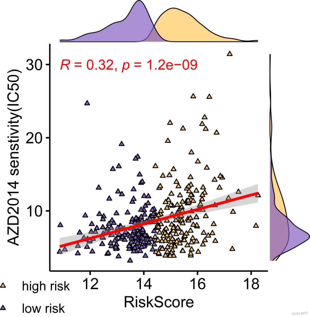
#Create risk score and sensitivity (IC50) correlation curves.
library(data.table)
testPtype <- fread(‘./calcPhenotype_Output/DrugPredictions.csv’, data.table = F)
row.names(testPtype) <- testPtype[,1]
testPtype<- testPtype[,-1]
testPtype$RiskScore <- RiskScore
testPtype <- t(testPtype)
#Grouping based on risk scores
Group <- ifelse(testPtype$RiskScore>=median(testPtype$RiskScore),’high risk’,’low risk’)
testPtype <- as.data.frame(testPtype)
type = levels(factor(Group))
comp=combn(type,2)
my_comparisons=list()
for (i in 1:ncol(comp)) {my_comparisons[[i]]<-comp[,i]}
### Correlation between batch calculation of risk scores and sensitivity (IC50)
batch_cor <- function(gene){
y <- as.numeric(testPtype[gene,])
rownames <- rownames(testPtype)
do.call(rbind,future_lapply(rownames, function(x){
dd <- cor.test(as.numeric(testPtype[x,]),y,type=”spearman”)
data.frame(gene=gene,mRNAs=x,cor=dd$estimate,p.value=dd$p.value )
}))
}
#Calculate the correlation between risk score and drug sensitivity
library(future.apply)
system.time(DRUG <- batch_cor(“RiskScore”))
#Draw correlation curve
library(ggpubr)
library(ggplot2)
plot <- ggscatterhist(
testPtype, x =”RiskScore”, y =”AZD2014_1441″,
shape=c(24),fill= “Group”, size =1, alpha = 2,
palette = c(“#FFC75F”, “#845EC2”),
margin.plot = “density”,
margin.params = list(fill = “Group”,size = 0.3),
legend = c(0.9,0.15))
plot$sp <- plot$sp +
stat_smooth(method=”lm”,se=TRUE,color=”red”)+stat_cor(data=testPtype, method = “pearson”,color=”red”)+
labs(x=”RiskScore”,y=paste0(“AZD2014″,” senstivity(IC50)”))#+theme_light()
plot
write.csv(DRUG,”./DRUG.csv”)